library(dplyr)
library(tidyverse)
library(jsonlite)
library(xtable)
library(data.table)E1_Power_Analysis
Plan for power analysis.
- Use data from E1B to estimate average proportion recalled per cell in the design.
- Use the proportion as probability for a binomial distribution.
- Simulate recall data in the design
- Estimate number of subjects needed for different effect sizes
Load libraries
Import Data
# Read the text file from JATOS ...
read_file('data/E1B_self_reference_deID.JSON') %>%
  # ... split it into lines ...
  str_split('\n') %>% first() %>%
  # ... filter empty rows ...
  discard(function(x) x == '') %>%
  # ... parse JSON into a data.frame
  map_dfr(fromJSON, flatten=T) -> all_data
Demographics
library(tidyr)

demographics <- all_data %>%
  filter(trial_type == "survey-html-form") %>%
  select(ID,response) %>%
  unnest_wider(response) %>%
  mutate(age = as.numeric(age))

age_demographics <- demographics %>%
  summarize(mean_age = mean(age),
            sd_age = sd(age),
            min_age = min(age),
            max_age = max(age))

factor_demographics <- apply(demographics[-1], 2, table)
Pre-processing
Case judgment accuracy
Get case judgment accuracy for all participants.
case_judgment <- all_data %>%
  filter(encoding_trial_type == "study_word",
         study_instruction == "case") %>%
  mutate(response = as.character(unlist(response))) %>%
  mutate(accuracy = case_when(
    response == "0" & letter_case == "upper" ~ 1,
    response == "1" & letter_case == "upper" ~ 0,
    response == "0" & letter_case == "lower" ~ 0,
    response == "1" & letter_case == "lower" ~ 1
         )) %>%
  group_by(ID) %>%
  summarise(percent_correct = mean(accuracy))

ggplot(case_judgment, aes(x=percent_correct))+
  geom_histogram() +
  geom_vline(xintercept=.7)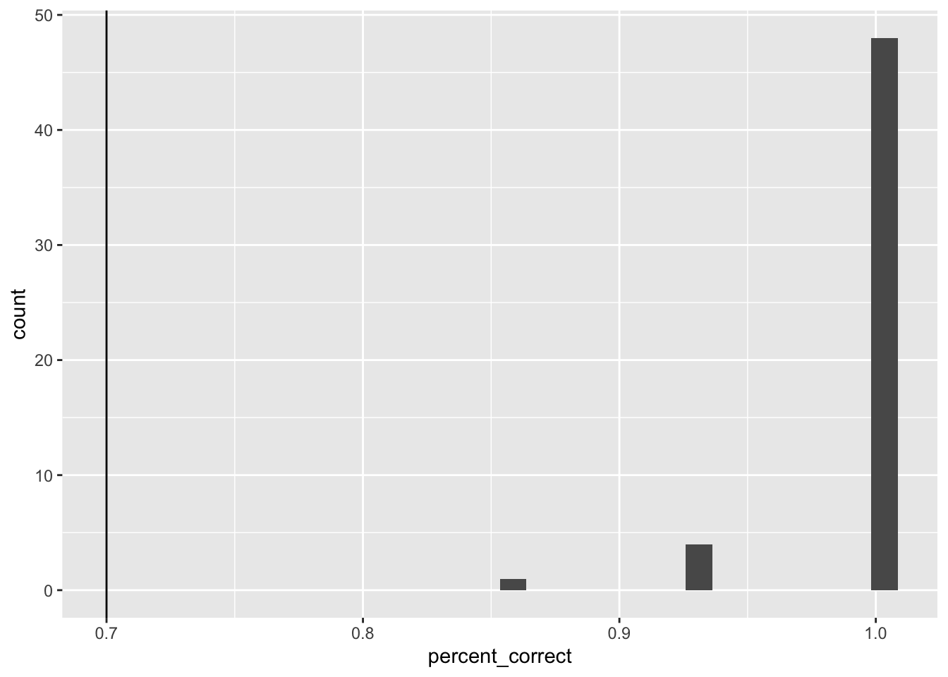
All exclusions
no exclusions
all_excluded <- case_judgment %>%
  filter(percent_correct < .7) %>%
  select(ID) %>%
  pull()

length(all_excluded)
[1] 0filtered_data <- all_data %>%
filter(ID %in% all_excluded == FALSE) Accuracy analysis
Define Helper functions
To do, consider moving the functions into the R package for this project
# attempt general solution

## Declare helper functions

################
# get_mean_sem
# data = a data frame
# grouping_vars = a character vector of factors for analysis contained in data
# dv = a string indicated the dependent variable colunmn name in data
# returns data frame with grouping variables, and mean_{dv}, sem_{dv}
# note: dv in mean_{dv} and sem_{dv} is renamed to the string in dv

get_mean_sem <- function(data, grouping_vars, dv, digits=3){
  a <- data %>%
    group_by_at(grouping_vars) %>%
    summarize("mean_{ dv }" := round(mean(.data[[dv]]), digits),
              "sem_{ dv }" := round(sd(.data[[dv]])/sqrt(length(.data[[dv]])),digits),
              .groups="drop")
  return(a)
}

################
# get_effect_names
# grouping_vars = a character vector of factors for analysis
# returns a named list
# list contains all main effects and interaction terms
# useful for iterating the computation means across design effects and interactions

get_effect_names <- function(grouping_vars){
  effect_names <- grouping_vars
  if( length(grouping_vars > 1) ){
    for( i in 2:length(grouping_vars) ){
      effect_names <- c(effect_names,apply(combn(grouping_vars,i),2,paste0,collapse=":"))
    }
  }
  effects <- strsplit(effect_names, split=":")
  names(effects) <- effect_names
  return(effects)
}

################
# print_list_of_tables
# table_list = a list of named tables
# each table is printed
# names are header level 3

print_list_of_tables <- function(table_list){
  for(i in 1:length(table_list)){
    cat("###",names(table_list[i]))
    cat("\n")
    print(knitr::kable(table_list[[i]]))
    cat("\n")
  }
}
Conduct Analysis
Recall Test Data
# obtain recall data from typed answers

recall_data <- filtered_data %>%
  filter(phase %in% c("recall_1","recall_2") == TRUE ) %>%
  select(ID,phase,paragraph) %>%
  pivot_wider(names_from = phase,
              values_from = paragraph) %>%
  mutate(recall_1 = paste(recall_1,recall_2,sep = " ")) %>%
  select(ID,recall_1) %>%
 # separate_longer_delim(cols = recall_1,
 #                        delim = " ") %>%
  mutate(recall_1 = tolower(recall_1)) %>%
  mutate(recall_1 = gsub("[^[:alnum:][:space:]]","",recall_1))

encoding_words_per_subject <- filtered_data %>%
  filter(encoding_trial_type == "study_word",
         phase == "main_study")

recall_data <- left_join(encoding_words_per_subject,recall_data,by = 'ID') %>%
  mutate(recall_1 = strsplit(recall_1," "))

# implement a spell-checking method

recall_success <- c()
min_string_distance <- c()
for(i in 1:dim(recall_data)[1]){
  recalled_words <- unlist(recall_data$recall_1[i])
  recalled_words <- recalled_words[recalled_words != ""]
  if (length(recalled_words) == 0 ) recalled_words <- "nonerecalled"
  recall_success[i] <- tolower(recall_data$target_word[i]) %in% recalled_words
  min_string_distance[i] <- min(sapply(recalled_words,FUN = function(x) {
  stringdist::stringdist(a=x,b = tolower(recall_data$target_word[i]), method = "lv")
}))
}

# recall proportion correct by subject

recall_data_subject <- recall_data %>%
  mutate(recall_success = recall_success,
         min_string_distance = min_string_distance) %>%
  mutate(close_recall = min_string_distance <= 2) %>%
  group_by(ID,study_instruction,encoding_recall,block_type) %>%
  summarise(number_recalled = sum(recall_success),
            number_close_recalled = sum(close_recall)) %>%
  ungroup() %>%
  mutate(proportion_recalled = case_when(encoding_recall == "no_recall" ~ number_close_recalled/6,
                                         encoding_recall == "recall" ~ number_close_recalled/6)) %>%
  mutate(ID = as.factor(ID),
         study_instruction = as.factor(study_instruction),
         encoding_recall = as.factor(encoding_recall),
         block_type = as.factor(block_type))

# power analysis parameters from empirical data
mean_p_recall_per_cell <- mean(recall_data_subject$proportion_recalled)
sd_p_recall_per_cell <- sd(recall_data_subject$proportion_recalled)
emp_dist_p_recall_per_cell <- recall_data_subject$proportion_recalled
Power-analysis
Very simple approach. Use the mean_p_recall_per_cell to generate data from a binomial distribution.
6 observations per cell (comparison between cells, simple effects)
# This number came from empirical data
mean_p_recall_per_cell <- .2

# create a tibble to store simulation results
sim_data <- tibble()

# simulation parameters
num_sims <- 200 # number of times to a run a simulated experiment
number_of_subs <- c(10,20,30,40,50,60,70,80,90,100,150,200)
effect_sizes <- c(.01,.02,.03,.04,.05,.1,.2)


# Loop to run all simulations for every parameter
for(n in number_of_subs) {
  print(n) # shows simulation progress in the console

  for (effect in effect_sizes) {
    p_vals <-
      rep(0, num_sims) # initialize variable to store p values from each experiment

    # run simulated experiments
    for (reps in 1:num_sims) {
      # A uses rbinom to simulated how many words a person remembers given the base probability
      A <-
        colMeans(replicate(n, rbinom(6, 1, mean_p_recall_per_cell)))

      # B adds the effect size to the base probability
      B <-
        colMeans(replicate(n, rbinom(
          6, 1, mean_p_recall_per_cell + effect
        )))

      # run a t-test to compare whether the two are different
      t_test <- t.test(A, B, paired = TRUE)

      # store the p-value in the vector
      p_vals[reps] <- t_test$p.value

    }

    # add the results to a tibble with one row
    sim_result <- tibble(
      subs = n,
      effect_size = effect,
      rep = reps,
      prop_p_value = length(p_vals[p_vals < .05]) / num_sims # this is proportion of significant experiments, or power
    )

    sim_data <- rbind(sim_data, sim_result)
  }
}
[1] 10
[1] 20
[1] 30
[1] 40
[1] 50
[1] 60
[1] 70
[1] 80
[1] 90
[1] 100
[1] 150
[1] 200# summarize the data for plotting
sim_data_means <- sim_data %>%
mutate(effect_size = as.factor(effect_size)) %>%
group_by(subs,effect_size) %>%
summarise(mean_proportion = mean(prop_p_value), .groups = 'drop')
# plot the data
ggplot(sim_data_means,
aes(x=subs,
y=mean_proportion,
group = effect_size,
color = effect_size)) +
geom_point()+
geom_line()+
ylab("Proportion of significant experiments (Power)")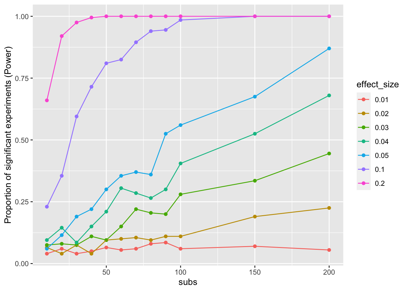
12 observations per cell: simple effects for main effect of levels of processing
sim_data <- tibble()

num_sims <- 200
number_of_subs <- c(10,20,30,40,50,60,70,80,90,100,150,200)
effect_sizes <- c(.01,.02,.03,.04,.05,.1,.2)

for(n in number_of_subs){
  print(n)
  for(effect in effect_sizes){
    p_vals <- rep(0,num_sims)
    for(reps in 1:num_sims){

      A <- colMeans(replicate(n, rbinom(12,1,mean_p_recall_per_cell)))
      B <- colMeans(replicate(n, rbinom(12,1,mean_p_recall_per_cell+effect)))

      t_test <- t.test(A,B,paired = TRUE)
      p_vals[reps] <- t_test$p.value
    }

     sim_result <- tibble(subs = n,
                           effect_size = effect,
                           rep = reps,
                           prop_p_value = length(p_vals[p_vals < .05])/num_sims)

      sim_data <- rbind(sim_data,sim_result)
  }
}
[1] 10
[1] 20
[1] 30
[1] 40
[1] 50
[1] 60
[1] 70
[1] 80
[1] 90
[1] 100
[1] 150
[1] 200sim_data_means <- sim_data %>%
mutate(effect_size = as.factor(effect_size)) %>%
group_by(subs,effect_size) %>%
summarise(mean_proportion = mean(prop_p_value), .groups = 'drop')
ggplot(sim_data_means,
aes(x=subs,
y=mean_proportion,
group = effect_size,
color = effect_size)) +
geom_point()+
geom_line()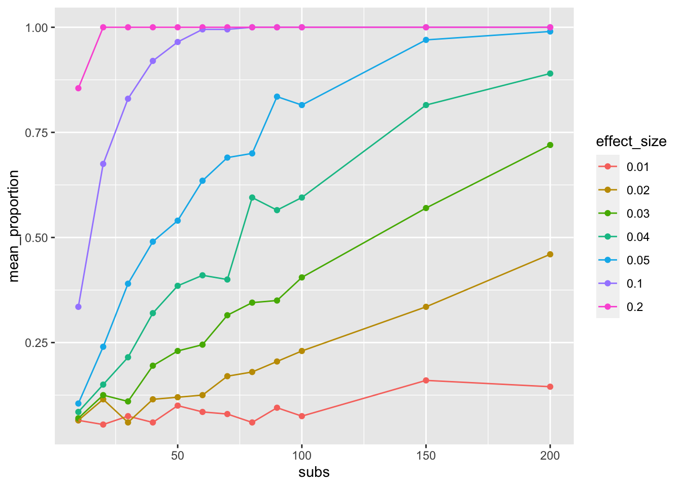
save data
save.image("data/E1_Power.RData")