Chapter 12 Animal Tracking with TRAJR

Author: Richard Troise

The R-package ‘Trajr’ had been recently implemented for biological research with the idea of tracking moving animals. Psychologists could make use of trajectories in animal learning studies, specifically when the animals utilize path integration. The tracking of an animal can first be recorded via video footage or GPS tracking. The data can then be imported in R, where it is transformed into a ‘trajectory’ object. The object itself contains: the trajectory data (as a data frame of coordinates and time steps), the time steps converted into a numerical unit, displacement information, and the polar coordinate-equivalent from Cartesian. From there, any user can choose to plot the trajectory and perform various calculations. The function ‘TrajDistance’ for examples, determines the shortest distance travelled based on the start and end point of a path.

The demonstration utilizes a custom function, built by the original author of Trajr, (???), to show what the general output looks like when calculating the variables ‘average speed’, ‘sinuosity’, and ‘straightness’. The speed is simply calculated as position over time. Sinuosity can be thought as how much curvature contributes to the total path relative to a shortest line connecting the two ‘start’ and ‘end’ points. The greater the number, the more bending of the path there is. The index of straightness is inferred by an ‘Emax’ value. Straighter paths hold higher values, and the range is allowed to approach infinity.

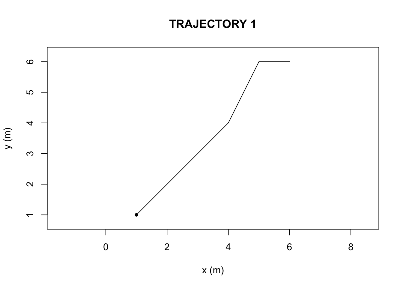
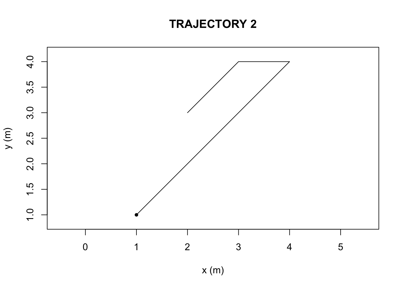
We first compiled two hypothetical trajectories in R-studio (Figure 1 and 2, Appendix), a data frame with a set of six x-coordinates (in units of meters), y-coordinates, and time steps (unitless). The ‘TrajFromCoords’ function, allows for the conversion of a data frame into a trajectory object. We then plotted the two objects to visualize the paths.

The function ‘characteriseTrajectory’ takes a single trajectory object and computes the average speed and standard deviation (that some animal would take) based on the derivatives calculated via ‘TrajDerivatives’. ‘TrajSinuosity’ and ‘TrajEmax’ are the functions that compute the sinuosity and straightness of the two paths. Lastly, the chracterizing function stores the computed information in the list which can be displayed at once or individually.

characteriseTrajectory <- function(trj) {
  # Measures of speed
  derivs <- TrajDerivatives(trj)
  mean_speed <- mean(derivs$speed)
  sd_speed <- sd(derivs$speed)
  
  # Measures of straightness
  sinuosity <- TrajSinuosity(trj)
  Emax <- TrajEmax(trj)
  
  # Return a list with all of the statistics for this trajectory
  list(mean_speed = mean_speed,
       sd_speed = sd_speed,
       sinuosity = sinuosity,
       Emax = Emax

  )
}

The sinuosity and E-max values were greater in Trajectory 2 than Trajectory 1.

Trajectory1	Parameter
74.7870866	Avg.Speed
22.5524852	Std.Speed
0.6038492	Sinuosity
5.6213862	Emax

Trajectory2	Parameter
66.568543	Avg.Speed
9.262097	Std.Speed
1.135893	Sinuosity
1.000000	Emax

Based on the outputs of the ‘characteriseTrajectory’, The first and second trajectories (Figure 1 and Figure 2) differ in their sinuosity and Emax due to the nature of the paths themselves. The bending behavior, is what causes the second trajectory, in Figure 2, to possess a higher turning value(sinuosity) and lower Emax (straightness) than in the first trajectory, in Figure 1. There is also a difference in speed parameters, but bending behavior is what can be visually and numerically ascertained.