E1_DF_Mixed • ForgettingPictures

Data collected 2/10/22

Load libraries

library(pacman)
library(dplyr)
library(tidyverse)
library(jsonlite)
library(xtable)
library(data.table)

Import Data

# Read the text file from JATOS ...
read_file('data/E1/jatos_results_20220330235250.txt') %>%
  # ... split it into lines ...
  str_split('\n') %>% first() %>%
  # ... filter empty rows ...
  discard(function(x) x == '') %>%
  # ... parse JSON into a data.frame
  map_dfr(fromJSON, flatten=T) -> all_data

Demographics

library(tidyr)

demographics <- all_data %>%
  filter(trial_type == "survey-html-form") %>%
  select(ID,response) %>%
  unnest_wider(response) %>%
  mutate(age = as.numeric(age))

age_demographics <- demographics %>%
  summarize(mean_age = mean(age),
            sd_age = sd(age),
            min_age = min(age),
            max_age = max(age))

factor_demographics <- apply(demographics[-1], 2, table)

A total of 47 participants were recruited from Amazon’s Mechanical Turk. Mean age was 34.9 (range = 22 to 60 ). There were 23 females, and 24 males. There were 41 right-handed participants, and NA left or both handed participants. 37 participants reported normal vision, and 10 participants reported corrected-to-normal vision. 37 participants reported English as a first language, and 10 participants reported English as a second language.

Pre-processing

We are interested in including participants who attempted to perform the task to the best of their ability. We adopted the following exclusion criteria.

Lower than 75% correct during the encoding task. This means that participants failed to correctly press the F or R keys on each trial.

# select data from the study phase
study_accuracy <- all_data %>%
  filter(experiment_phase == "study",
         is.na(correct) == FALSE) %>%
  group_by(ID)%>%
  summarize(mean_correct = mean(correct))

study_excluded_subjects <- study_accuracy %>%
  filter(mean_correct < .75) %>%
  pull(ID)

ggplot(study_accuracy, aes(x=mean_correct))+
  coord_cartesian(xlim=c(0,1))+
  geom_vline(xintercept=.75)+
  geom_histogram()+
  ggtitle("Histogram of mean correct responses \n for each subject during study phase")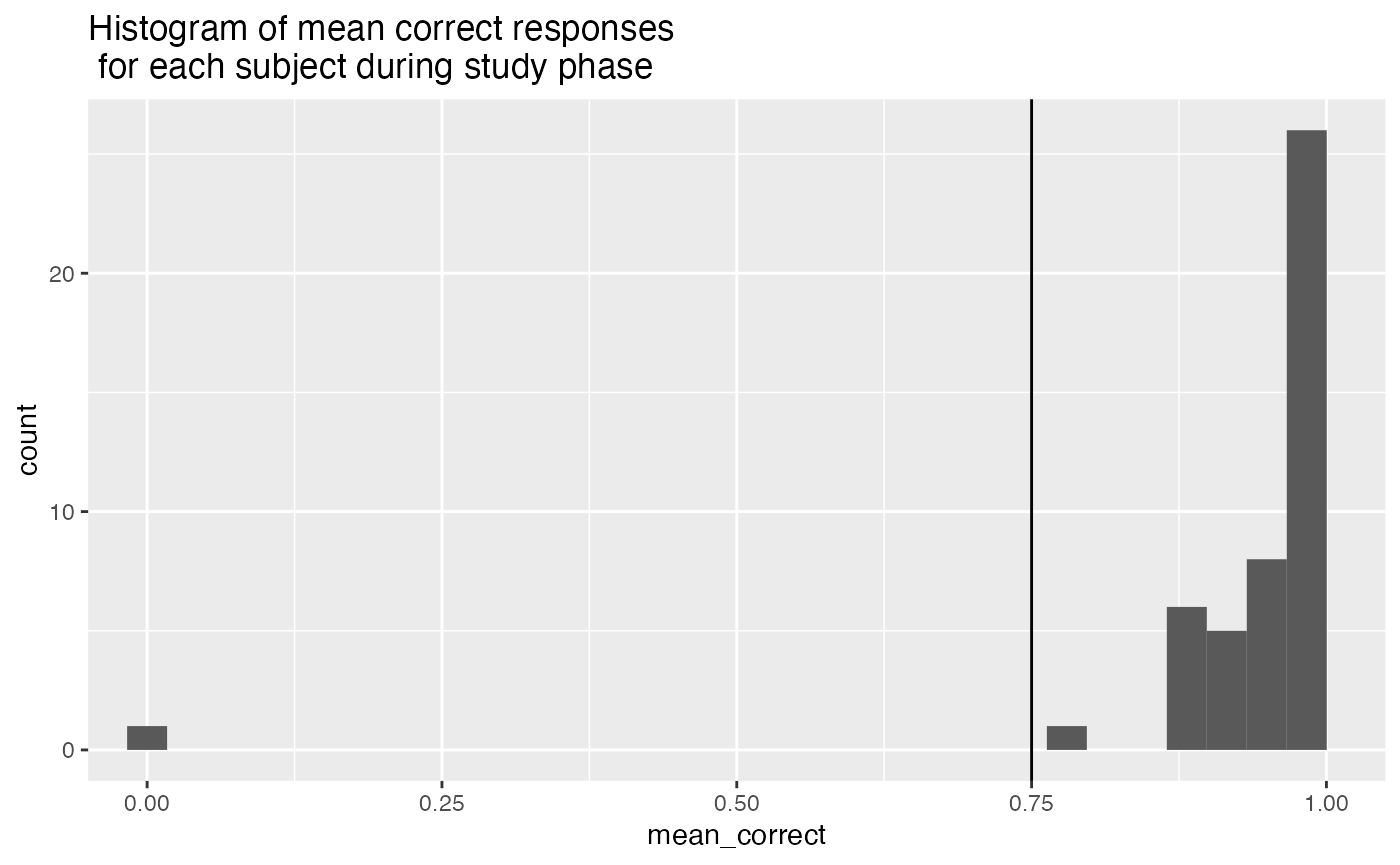

More than 25% Null responses (120*.25 = 30) during test. NULL responses mean that the participant did not respond on a test trial after 10 seconds.

# select data from the study phase
test_null <- all_data %>%
  filter(experiment_phase == "test",
         response =="NULL") %>%
  group_by(ID) %>%
  count()

test_null_excluded <- test_null %>%
  filter(n > (120*.25)) %>%
  pull(ID)

ggplot(test_null, aes(x=n))+
  geom_vline(xintercept=30)+
  geom_histogram()+
  ggtitle("Histogram of count of null responses \n for each subject during test")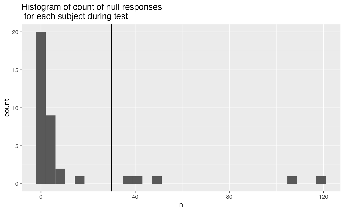

Higher than 75% response bias in the recognition task. This suggests that participants were simply pressing the same button on most trials.

test_response_bias <- all_data %>%
  filter(experiment_phase == "test",
         response !="NULL") %>%
  mutate(response = as.numeric(response)) %>%
  group_by(ID, response) %>%
  count() %>%
  pivot_wider(names_from = response,
              values_from = n,
              values_fill = 0) %>%
  mutate(bias = abs(`0` - `1`)/120)

test_response_bias_excluded <- test_response_bias %>%
  filter(bias > .75) %>%
  pull(ID)

ggplot(test_response_bias, aes(x=bias))+
  geom_vline(xintercept=.75)+
  geom_histogram()+
  ggtitle("Histogram of response bias \n for each subject during test phase")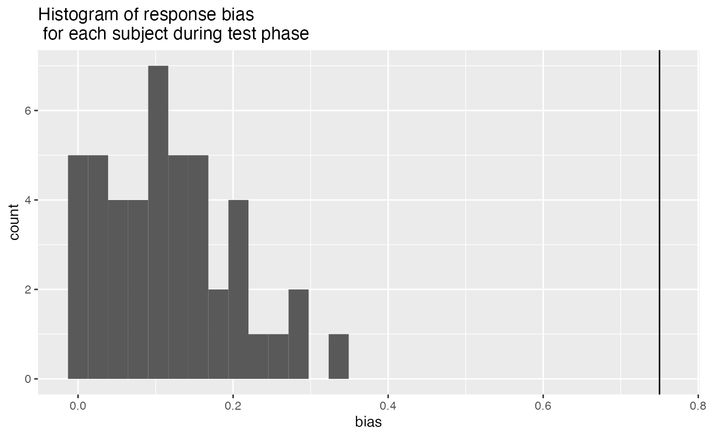

Making responses too fast during the recognition memory test, indicating that they weren’t performing the task. We excluded participants whose mean RT was less than 300 ms.

test_mean_rt <- all_data %>%
  filter(experiment_phase == "test",
         response !="NULL",
         rt != "NULL") %>%
  mutate(rt = as.numeric(rt)) %>%
  group_by(ID) %>%
  summarize(mean_RT = mean(rt))

test_mean_rt_excluded <- test_mean_rt %>%
  filter(mean_RT < 300) %>%
  pull(ID)

ggplot(test_mean_rt, aes(x=mean_RT))+
  geom_vline(xintercept=300)+
  geom_histogram()+
  ggtitle("Histogram of response bias \n for each subject during test phase")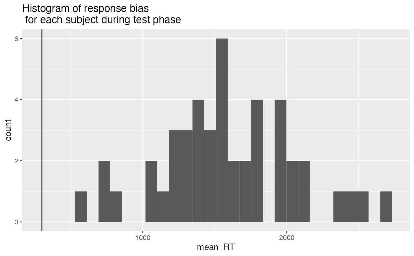

Subjects are included if they perform better than 55% correct on the novel lures.

test_mean_novel_accuracy <- all_data %>%
  filter(experiment_phase == "test",
         test_condition == "novel") %>%
  mutate(correct = as.logical(correct)) %>%
  group_by(ID) %>%
  summarize(mean_correct = mean(correct))

test_mean_novel_accuracy_excluded <- test_mean_novel_accuracy %>%
  filter(mean_correct < .55) %>%
  pull(ID)

ggplot(test_mean_novel_accuracy, aes(x=mean_correct))+
  geom_vline(xintercept=.55)+
  geom_histogram()+
  ggtitle("Histogram of mean accuracy for novel lures \n for each subject during test phase")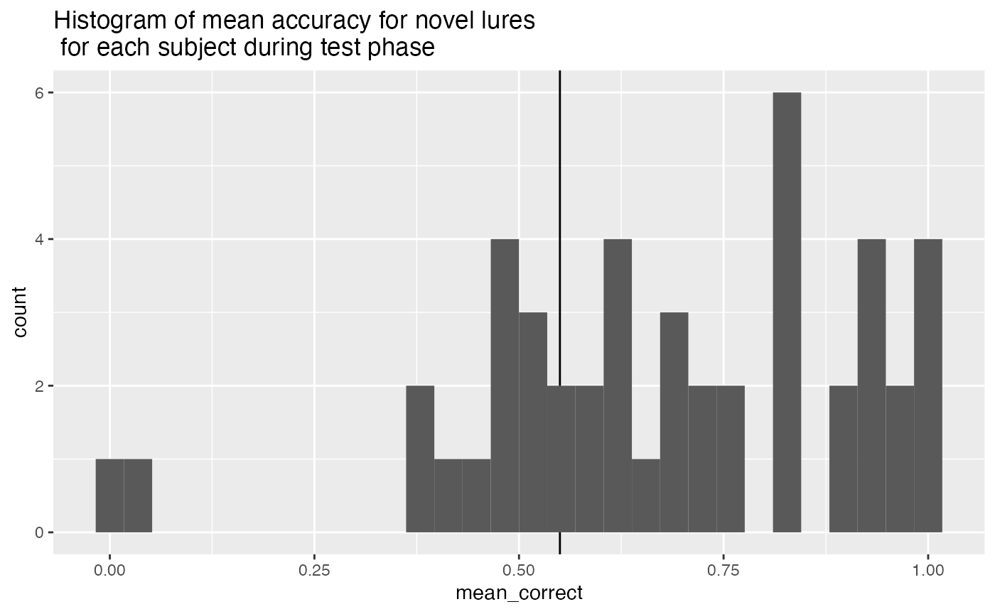

All exclusions

all_excluded <- unique(c(study_excluded_subjects,
                  test_null_excluded,
                  test_response_bias_excluded,
                  test_mean_rt_excluded,
                  test_mean_novel_accuracy_excluded))

length(all_excluded)

## [1] 13

Our participants were recruited online and completed the experiment from a web browser. Our experiment script requests that participants attempt the task to the best of their ability. Nevertheless, it is possible that participants complete the experiment and submit data without attempting to complete the task as directed. We developed a set of criteria to exclude participants whose performance indicated they were not attempting the task as instructed. These criteria also allowed us to confirm that the participants we included in the analysis did attempt the task as instructed to the best of their ability. We adopted the following five criteria:

First, during the encoding phase participants responded to each instructional cue (to remember or forget the picture on each trial) by pressing “R” or “F” on the keyboard. This task demand further served as an attentional check. We excluded participants who scored lower than 75% correct on instructional cue identification responses. Second, participants who did not respond on more than 25% of trials in the recognition test were excluded. Third, we measured response bias (choosing the left or right picture) during the recognition test, and excluded participants who made 75% of their responses to one side (indicating they were repeatedly pressing the same button on each trial). Fourth, we excluded participants whose mean reaction time during the recognition test was less than 300ms, indicating they were pressing the buttons as fast as possible without making a recognition decision. Finally, we computed mean accuracy for the novel lure condition for all participants, and excluded participants whose mean accuracy was less than 55% for those items. All together 13 participants were excluded.

Accuracy analysis

Define Helper functions

To do, consider moving the functions into the R package for this project

# attempt general solution

## Declare helper functions

################
# get_mean_sem
# data = a data frame
# grouping_vars = a character vector of factors for analysis contained in data
# dv = a string indicated the dependent variable colunmn name in data
# returns data frame with grouping variables, and mean_{dv}, sem_{dv}
# note: dv in mean_{dv} and sem_{dv} is renamed to the string in dv

get_mean_sem <- function(data, grouping_vars, dv, digits=3){
  a <- data %>%
    group_by_at(grouping_vars) %>%
    summarize("mean_{ dv }" := round(mean(.data[[dv]]), digits),
              "sem_{ dv }" := round(sd(.data[[dv]])/sqrt(length(.data[[dv]])),digits),
              .groups="drop")
  return(a)
}

################
# get_effect_names
# grouping_vars = a character vector of factors for analysis
# returns a named list
# list contains all main effects and interaction terms
# useful for iterating the computation means across design effects and interactions

get_effect_names <- function(grouping_vars){
  effect_names <- grouping_vars
  if( length(grouping_vars > 1) ){
    for( i in 2:length(grouping_vars) ){
      effect_names <- c(effect_names,apply(combn(grouping_vars,i),2,paste0,collapse=":"))
    }
  }
  effects <- strsplit(effect_names, split=":")
  names(effects) <- effect_names
  return(effects)
}

################
# print_list_of_tables
# table_list = a list of named tables
# each table is printed 
# names are header level 3

print_list_of_tables <- function(table_list){
  for(i in 1:length(table_list)){
    cat("###",names(table_list[i]))
    cat("\n")
    print(knitr::kable(table_list[[i]]))
    cat("\n")
  }
}

Conduct Analysis

# create list to hold results
Accuracy <- list()

# Pre-process data for analysis
# assign to "filtered_data" object
Accuracy$filtered_data <- all_data %>%
  filter(experiment_phase == "test", 
         ID %in% all_excluded == FALSE)

# declare factors, IVS, subject variable, and DV
Accuracy$factors$IVs <- c("encoding_stimulus_time",
                          "encoding_instruction",
                          "test_condition")
Accuracy$factors$subject <- "ID"
Accuracy$factors$DV <- "correct"

## Subject-level means used for ANOVA
# get individual subject means for each condition
Accuracy$subject_means <- get_mean_sem(data=Accuracy$filtered_data,
                                       grouping_vars = c(Accuracy$factors$subject,
                                                         Accuracy$factors$IVs),
                                       dv = Accuracy$factors$DV)
## Condition-level means
# get all possible main effects and interactions
Accuracy$effects <- get_effect_names(Accuracy$factors$IVs)

Accuracy$means <- lapply(Accuracy$effects, FUN = function(x) {
  get_mean_sem(data=Accuracy$filtered_data,
             grouping_vars = x,
             dv = Accuracy$factors$DV)
})

## ANOVA

# ensure factors are factor class
Accuracy$subject_means <- Accuracy$subject_means %>%
  mutate_at(Accuracy$factors$IVs,factor) %>%
  mutate_at(Accuracy$factors$subject,factor)

# run ANOVA
Accuracy$aov.out <- aov(mean_correct ~ encoding_stimulus_time*encoding_instruction*test_condition + Error(ID/(encoding_stimulus_time*encoding_instruction*test_condition)), Accuracy$subject_means)

# save printable summaries
Accuracy$apa_print <- papaja::apa_print(Accuracy$aov.out)

Graphs

Accuracy$graphs$figure <- ggplot(Accuracy$means$`encoding_stimulus_time:encoding_instruction:test_condition`, 
                                 aes(x=test_condition,
                                     y=mean_correct,
                                     group=encoding_instruction,
                                     fill=encoding_instruction))+
  geom_bar(stat="identity", position="dodge")+
  geom_errorbar(aes(ymin = mean_correct-sem_correct,
                    ymax = mean_correct+sem_correct),
                width=.9, position=position_dodge2(width = 0.2, padding = 0.8))+
  facet_wrap(~encoding_stimulus_time)+
  coord_cartesian(ylim=c(.4,1))+
  geom_hline(yintercept=.5)+
  scale_y_continuous(breaks = seq(0.4,1,.1))+
  theme_classic(base_size=12)+
  ylab("Proportion Correct")+
  xlab("Lure Type")+
  scale_fill_discrete(name = " Encoding \n Instruction") +
  ggtitle("E1: Proportion Correct by Stimulus Encoding Duration, \n Encoding Instruction, and Lure Type")

Accuracy$graphs$figure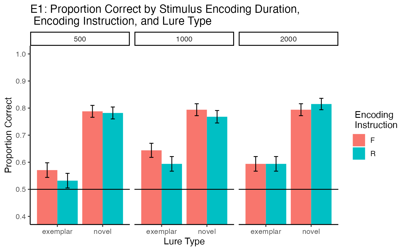

Print ANOVA

knitr::kable(xtable(summary(Accuracy$aov.out)))

	Df	Sum Sq	Mean Sq	F value	Pr(>F)
Residuals	33	4.7925490	0.1452288	NA	NA
encoding_stimulus_time	2	0.0885784	0.0442892	2.6182656	0.0804931
Residuals	66	1.1164216	0.0169155	NA	NA
encoding_instruction	1	0.0283333	0.0283333	1.9547038	0.1714078
Residuals	33	0.4783333	0.0144949	NA	NA
test_condition	1	4.1603922	4.1603922	133.3448867	0.0000000
Residuals	33	1.0296078	0.0312002	NA	NA
encoding_stimulus_time:encoding_instruction	2	0.0415196	0.0207598	0.9470100	0.3931059
Residuals	66	1.4468137	0.0219214	NA	NA
encoding_stimulus_time:test_condition	2	0.0918137	0.0459069	2.9904204	0.0571205
Residuals	66	1.0131863	0.0153513	NA	NA
encoding_instruction:test_condition	1	0.0165686	0.0165686	1.2423702	0.2730668
Residuals	33	0.4400980	0.0133363	NA	NA
encoding_stimulus_time:encoding_instruction:test_condition	2	0.0006373	0.0003186	0.0121719	0.9879041
Residuals	66	1.7276961	0.0261772	NA	NA

Print Means

print_list_of_tables(Accuracy$means)

encoding_stimulus_time

encoding_stimulus_time	mean_correct	sem_correct
500	0.668	0.013
1000	0.700	0.012
2000	0.699	0.012

encoding_instruction

encoding_instruction	mean_correct	sem_correct
F	0.698	0.01
R	0.681	0.01

test_condition

test_condition	mean_correct	sem_correct
exemplar	0.588	0.011
novel	0.790	0.009

encoding_stimulus_time:encoding_instruction

encoding_stimulus_time	encoding_instruction	mean_correct	sem_correct
500	F	0.679	0.018
500	R	0.657	0.018
1000	F	0.719	0.017
1000	R	0.681	0.018
2000	F	0.694	0.018
2000	R	0.704	0.018

encoding_stimulus_time:test_condition

encoding_stimulus_time	test_condition	mean_correct	sem_correct
500	exemplar	0.551	0.019
500	novel	0.785	0.016
1000	exemplar	0.619	0.019
1000	novel	0.781	0.016
2000	exemplar	0.594	0.019
2000	novel	0.804	0.015

encoding_instruction:test_condition

encoding_instruction	test_condition	mean_correct	sem_correct
F	exemplar	0.603	0.015
F	novel	0.792	0.013
R	exemplar	0.574	0.015
R	novel	0.788	0.013

encoding_stimulus_time:encoding_instruction:test_condition

encoding_stimulus_time	encoding_instruction	test_condition	mean_correct	sem_correct
500	F	exemplar	0.571	0.027
500	F	novel	0.788	0.022
500	R	exemplar	0.532	0.027
500	R	novel	0.782	0.022
1000	F	exemplar	0.644	0.026
1000	F	novel	0.794	0.022
1000	R	exemplar	0.594	0.027
1000	R	novel	0.768	0.023
2000	F	exemplar	0.594	0.027
2000	F	novel	0.794	0.022
2000	R	exemplar	0.594	0.027
2000	R	novel	0.815	0.021

Comparisons

## Encoding time x instruction
Accuracy$simple$DF_500 <- Accuracy$subject_means %>%
  filter(encoding_stimulus_time == "500") %>%
  group_by(ID,encoding_instruction) %>%
  summarize(mean_correct = mean(mean_correct)) %>%
  pivot_wider(names_from = encoding_instruction,
              values_from = mean_correct) %>%
  mutate(difference = R-F) %>%
  pull(difference) %>%
  t.test() %>%
  papaja::apa_print()

Accuracy$simple$DF_1000 <- Accuracy$subject_means %>%
  filter(encoding_stimulus_time == "1000") %>%
  group_by(ID,encoding_instruction) %>%
  summarize(mean_correct = mean(mean_correct)) %>%
  pivot_wider(names_from = encoding_instruction,
              values_from = mean_correct) %>%
  mutate(difference = R-F) %>%
  pull(difference) %>%
  t.test() %>%
  papaja::apa_print()

Accuracy$simple$DF_2000 <- Accuracy$subject_means %>%
  filter(encoding_stimulus_time == "2000") %>%
  group_by(ID,encoding_instruction) %>%
  summarize(mean_correct = mean(mean_correct)) %>%
  pivot_wider(names_from = encoding_instruction,
              values_from = mean_correct) %>%
  mutate(difference = R-F) %>%
  pull(difference) %>%
  t.test() %>%
  papaja::apa_print()

# encoding time x test condition

Accuracy$simple$test_500 <- Accuracy$subject_means %>%
  filter(encoding_stimulus_time == "500") %>%
  group_by(ID,test_condition) %>%
  summarize(mean_correct = mean(mean_correct)) %>%
  pivot_wider(names_from = test_condition,
              values_from = mean_correct) %>%
  mutate(difference = novel-exemplar) %>%
  pull(difference) %>%
  t.test() %>%
  papaja::apa_print()

Accuracy$simple$test_1000 <- Accuracy$subject_means %>%
  filter(encoding_stimulus_time == "1000") %>%
  group_by(ID,test_condition) %>%
  summarize(mean_correct = mean(mean_correct)) %>%
  pivot_wider(names_from = test_condition,
              values_from = mean_correct) %>%
  mutate(difference = novel-exemplar) %>%
  pull(difference) %>%
  t.test() %>%
  papaja::apa_print()

Accuracy$simple$test_2000 <- Accuracy$subject_means %>%
  filter(encoding_stimulus_time == "2000") %>%
  group_by(ID,test_condition) %>%
  summarize(mean_correct = mean(mean_correct)) %>%
  pivot_wider(names_from = test_condition,
              values_from = mean_correct) %>%
  mutate(difference = novel-exemplar) %>%
  pull(difference) %>%
  t.test() %>%
  papaja::apa_print()

Write-up

## helper print functions
qprint <- function(data,iv,level,dv){
   data[[iv]] %>%
   filter(.data[[iv]] == {level}) %>%
   pull(dv)
}

qprint_mean_sem <- function(data,iv,level,dv){
   dv_mean <- data[[iv]] %>%
   filter(.data[[iv]] == {level}) %>%
   pull(dv[1])
   
   dv_sem <- data[[iv]] %>%
   filter(.data[[iv]] == {level}) %>%
   pull(dv[2])
   
   return(paste("M = ", 
    dv_mean,
    ", SEM = ",
    dv_sem,
    sep=""))
   
}

# qprint(Accuracy$means,"encoding_stimulus_time","500","mean_correct")
# qprint_mean_sem(Accuracy$means,"encoding_stimulus_time","500",c("mean_correct","sem_correct"))

# use data.table for interactions

#t <- as.data.table(Accuracy$means$`encoding_stimulus_time:encoding_instruction`)
#t[encoding_stimulus_time==500 & encoding_instruction == "F"]$mean_correct

Proportion correct for each subject in each condition was submitted to a 3 (Encoding Duration: 500ms, 1000ms, 2000ms) x 2 (Encoding Instruction: Forget vs. Remember) x 2 (Lure type: Novel vs. Exemplar) fully repeated measures ANOVA. For completeness, each main effect and higher-order interaction is described in turn.

The main effect of encoding duration was not significant, \(F(2, 66) = 2.62\), \(p = .080\), \(\hat{\eta}^2_G = .007\), 90% CI \([.000, .048]\). Proportion correct was similar across the 500 ms (M = 0.668, SEM = 0.013), 1000 ms (M = 0.7, SEM = 0.012), and 2000 ms (M = 0.699, SEM = 0.012) stimulus durations.

The main effect of encoding instruction was not significant, \(F(1, 33) = 1.95\), \(p = .171\), \(\hat{\eta}^2_G = .002\), 90% CI \([.000, .005]\). Proportion correct was similar for remember cues (M = 0.681, SEM = 0.01) and forget cues (M = 0.698, SEM = 0.01).

The main effect of lure type was significant, \(F(1, 33) = 133.34\), \(p < .001\), \(\hat{\eta}^2_G = .257\), 90% CI \([.070, .444]\). Proportion correct was higher for novel lures (M = 0.79, SEM = 0.009) than exemplar lures (M = 0.588, SEM = 0.011).

The main question of interest was whether directing forgetting would vary across the encoding duration times. The interaction between encoding instruction and encoding duration was, \(F(2, 66) = 0.95\), \(p = .393\), \(\hat{\eta}^2_G = .003\), 90% CI \([.000, .024]\).

Paired sample t-tests were used to assess the directed forgetting effect at each encoding duration. The directed forgetting effect is taken as the difference between proportion correct for remember minus forget items. At 500 ms, the directed forgetting effect was reversed and not significant, \(M = -0.02\), 95% CI \([-0.07, 0.03]\), \(t(33) = -0.86\), \(p = .398\). At 1000ms, the directed forgetting effect was reversed and not significant, \(M = -0.04\), 95% CI \([-0.09, 0.01]\), \(t(33) = -1.61\), \(p = .118\). And, at 2000 ms, the directed forgetting effect was again not detected, \(M = 0.01\), 95% CI \([-0.03, 0.06]\), \(t(33) = 0.47\), \(p = .643\).

The encoding duration by lure type interaction was, \(F(2, 66) = 2.99\), \(p = .057\), \(\hat{\eta}^2_G = .008\), 90% CI \([.000, .049]\). In the 500 ms condition, proportion correct was higher for novel than exemplar lures, \(M = 0.23\), 95% CI \([0.19, 0.28]\), \(t(33) = 10.00\), \(p < .001\). The advantage for novel over exemplar items was smaller in the 1000 ms condition, \(M = 0.16\), 95% CI \([0.11, 0.21]\), \(t(33) = 6.80\), \(p < .001\), and 2000 ms condition \(M = 0.21\), 95% CI \([0.16, 0.26]\), \(t(33) = 7.91\), \(p < .001\).

The encoding instruction by lure type interaction was not significant, \(F(1, 33) = 1.24\), \(p = .273\), \(\hat{\eta}^2_G = .001\), 90% CI \([.000, .069]\). Similarly, the interaction between encoding duration, instruction, and lure type was not significant, \(F(2, 66) = 0.01\), \(p = .988\), \(\hat{\eta}^2_G = .000\), 90% CI \([.000, .000]\).

Reaction Time Analysis

Conduct Analysis

# create list to hold results
RT <- list()

# Pre-process data for analysis
# assign to "filtered_data" object
RT$filtered_data <- all_data %>%
  filter(experiment_phase == "test", 
         ID %in% all_excluded == FALSE,
         rt != "NULL") %>%
  mutate(rt = as.numeric(rt))

# declare factors, IVS, subject variable, and DV
RT$factors$IVs <- c("encoding_stimulus_time",
                          "encoding_instruction",
                          "test_condition")
RT$factors$subject <- "ID"
RT$factors$DV <- "rt"

## Subject-level means used for ANOVA
# get individual subject means for each condition
RT$subject_means <- get_mean_sem(data=RT$filtered_data,
                                       grouping_vars = c(RT$factors$subject,
                                                         RT$factors$IVs),
                                       dv = RT$factors$DV)
## Condition-level means
# get all possible main effects and interactions
RT$effects <- get_effect_names(RT$factors$IVs)

RT$means <- lapply(RT$effects, FUN = function(x) {
  get_mean_sem(data=RT$filtered_data,
             grouping_vars = x,
             dv = RT$factors$DV)
})

## ANOVA

# ensure factors are factor class
RT$subject_means <- RT$subject_means %>%
  mutate_at(RT$factors$IVs,factor) %>%
  mutate_at(RT$factors$subject,factor)

# run ANOVA
RT$aov.out <- aov(mean_rt ~ encoding_stimulus_time*encoding_instruction*test_condition + Error(ID/(encoding_stimulus_time*encoding_instruction*test_condition)), RT$subject_means)

# save printable summaries
RT$apa_print <- papaja::apa_print(RT$aov.out)

Graphs

RT$graphs$figure <- ggplot(RT$means$`encoding_stimulus_time:encoding_instruction:test_condition`, 
                                 aes(x=test_condition,
                                     y=mean_rt,
                                     group=encoding_instruction,
                                     fill=encoding_instruction))+
  geom_bar(stat="identity", position="dodge")+
  geom_errorbar(aes(ymin = mean_rt-sem_rt,
                    ymax = mean_rt+sem_rt),
                width=.9, position=position_dodge2(width = 0.2, padding = 0.8))+
  facet_wrap(~encoding_stimulus_time)+
  coord_cartesian(ylim=c(1000,2000))+
  scale_y_continuous(breaks = seq(1000,2000,100))+
  theme_classic(base_size=12)+
  ylab("Mean RT (ms)")+
  xlab("Lure Type")+
  scale_fill_discrete(name = " Encoding \n Instruction") +
  ggtitle("E1: Mean RT by Stimulus Encoding Duration, \n Encoding Instruction, and Lure Type")

RT$graphs$figure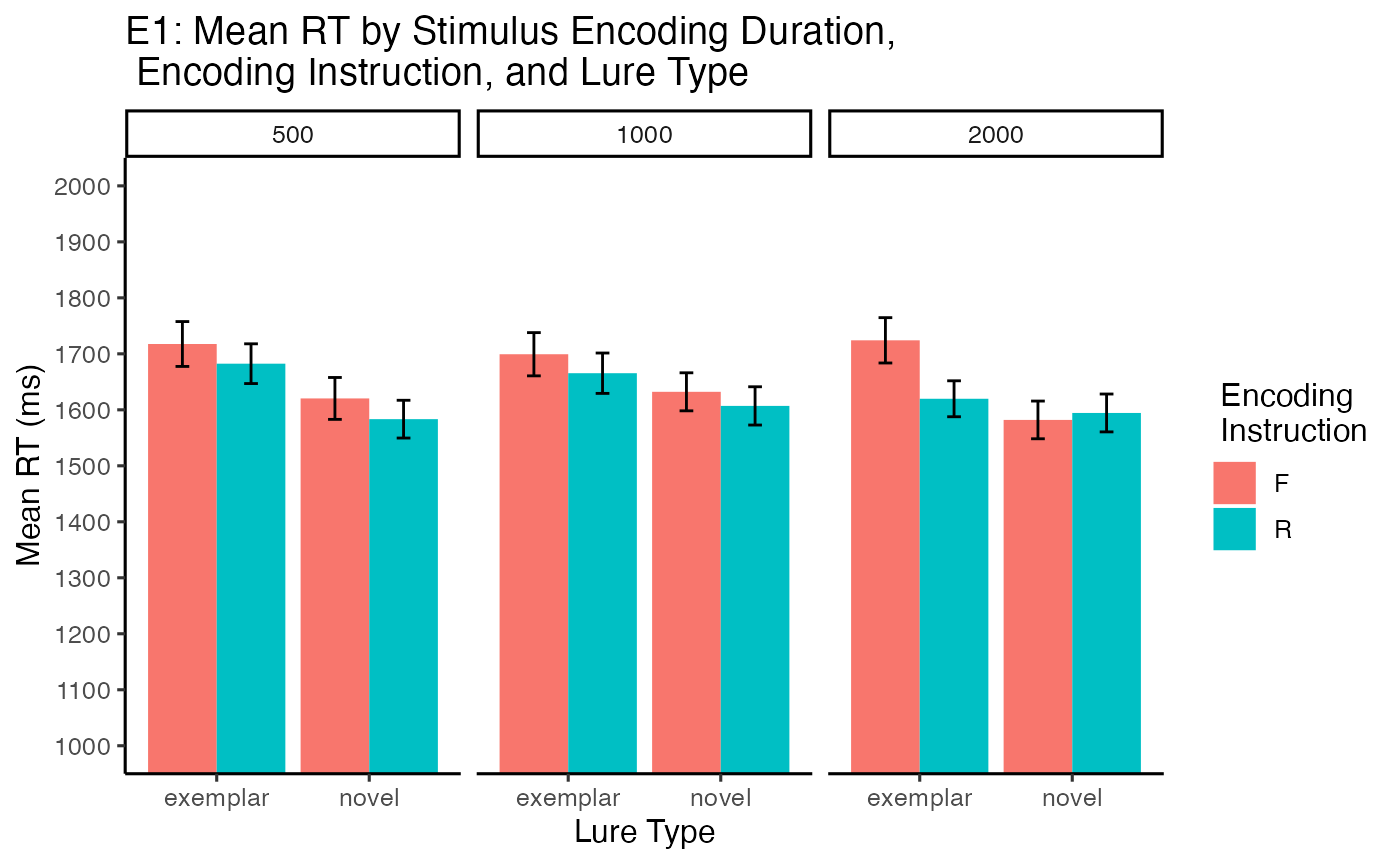

Print ANOVA

knitr::kable(xtable(summary(RT$aov.out)))

	Df	Sum Sq	Mean Sq	F value	Pr(>F)
Residuals	33	42156245.885	1277461.997	NA	NA
encoding_stimulus_time	2	30341.855	15170.928	0.4795306	0.6212139
Residuals	66	2088044.555	31637.039	NA	NA
encoding_instruction	1	177573.172	177573.172	5.4367884	0.0259695
Residuals	33	1077826.505	32661.409	NA	NA
test_condition	1	604114.759	604114.759	6.7383947	0.0139775
Residuals	33	2958536.560	89652.623	NA	NA
encoding_stimulus_time:encoding_instruction	2	2582.818	1291.409	0.0415036	0.9593709
Residuals	66	2053626.396	31115.551	NA	NA
encoding_stimulus_time:test_condition	2	25851.951	12925.976	0.3841409	0.6825481
Residuals	66	2220837.224	33649.049	NA	NA
encoding_instruction:test_condition	1	57136.209	57136.209	1.2656738	0.2686962
Residuals	33	1489716.354	45142.920	NA	NA
encoding_stimulus_time:encoding_instruction:test_condition	2	71921.183	35960.592	1.1484839	0.3233724
Residuals	66	2066549.737	31311.360	NA	NA

Print Means

print_list_of_tables(RT$means)

encoding_stimulus_time

encoding_stimulus_time	mean_rt	sem_rt
500	1650.684	18.405
1000	1650.887	17.881
2000	1630.329	17.658

encoding_instruction

encoding_instruction	mean_rt	sem_rt
F	1662.582	15.328
R	1625.191	13.987

test_condition

test_condition	mean_rt	sem_rt
exemplar	1684.996	15.225
novel	1603.181	14.070

encoding_stimulus_time:encoding_instruction

encoding_stimulus_time	encoding_instruction	mean_rt	sem_rt
500	F	1668.729	27.447
500	R	1632.639	24.530
1000	F	1665.714	25.728
1000	R	1635.926	24.835
2000	F	1653.363	26.477
2000	R	1606.984	23.309

encoding_stimulus_time:test_condition

encoding_stimulus_time	test_condition	mean_rt	sem_rt
500	exemplar	1699.975	26.751
500	novel	1601.832	25.177
1000	exemplar	1682.482	26.421
1000	novel	1619.575	24.079
2000	exemplar	1672.553	25.967
2000	novel	1588.167	23.847

encoding_instruction:test_condition

encoding_instruction	test_condition	mean_rt	sem_rt
F	exemplar	1713.690	22.923
F	novel	1611.474	20.238
R	exemplar	1655.898	19.969
R	novel	1594.880	19.559

encoding_stimulus_time:encoding_instruction:test_condition

encoding_stimulus_time	encoding_instruction	test_condition	mean_rt	sem_rt
500	F	exemplar	1717.554	40.068
500	F	novel	1620.339	37.417
500	R	exemplar	1682.396	35.490
500	R	novel	1583.324	33.723
1000	F	exemplar	1699.271	38.618
1000	F	novel	1632.158	33.964
1000	R	exemplar	1665.387	36.053
1000	R	novel	1606.993	34.178
2000	F	exemplar	1724.132	40.490
2000	F	novel	1581.961	33.678
2000	R	exemplar	1619.728	32.100
2000	R	novel	1594.392	33.818

Comparisons

## Encoding time x instruction
RT$simple$DF_500 <- RT$subject_means %>%
  filter(encoding_stimulus_time == "500") %>%
  group_by(ID,encoding_instruction) %>%
  summarize(mean_rt = mean(mean_rt)) %>%
  pivot_wider(names_from = encoding_instruction,
              values_from = mean_rt) %>%
  mutate(difference = R-F) %>%
  pull(difference) %>%
  t.test() %>%
  papaja::apa_print()

RT$simple$DF_1000 <- RT$subject_means %>%
  filter(encoding_stimulus_time == "1000") %>%
  group_by(ID,encoding_instruction) %>%
  summarize(mean_rt = mean(mean_rt)) %>%
  pivot_wider(names_from = encoding_instruction,
              values_from = mean_rt) %>%
  mutate(difference = R-F) %>%
  pull(difference) %>%
  t.test() %>%
  papaja::apa_print()

RT$simple$DF_2000 <- RT$subject_means %>%
  filter(encoding_stimulus_time == "2000") %>%
  group_by(ID,encoding_instruction) %>%
  summarize(mean_rt = mean(mean_rt)) %>%
  pivot_wider(names_from = encoding_instruction,
              values_from = mean_rt) %>%
  mutate(difference = R-F) %>%
  pull(difference) %>%
  t.test() %>%
  papaja::apa_print()

# encoding time x test condition

RT$simple$test_500 <- RT$subject_means %>%
  filter(encoding_stimulus_time == "500") %>%
  group_by(ID,test_condition) %>%
  summarize(mean_rt = mean(mean_rt)) %>%
  pivot_wider(names_from = test_condition,
              values_from = mean_rt) %>%
  mutate(difference = novel-exemplar) %>%
  pull(difference) %>%
  t.test() %>%
  papaja::apa_print()

RT$simple$test_1000 <- RT$subject_means %>%
  filter(encoding_stimulus_time == "1000") %>%
  group_by(ID,test_condition) %>%
  summarize(mean_rt = mean(mean_rt)) %>%
  pivot_wider(names_from = test_condition,
              values_from = mean_rt) %>%
  mutate(difference = novel-exemplar) %>%
  pull(difference) %>%
  t.test() %>%
  papaja::apa_print()

RT$simple$test_2000 <- RT$subject_means %>%
  filter(encoding_stimulus_time == "2000") %>%
  group_by(ID,test_condition) %>%
  summarize(mean_rt = mean(mean_rt)) %>%
  pivot_wider(names_from = test_condition,
              values_from = mean_rt) %>%
  mutate(difference = novel-exemplar) %>%
  pull(difference) %>%
  t.test() %>%
  papaja::apa_print()

Write-up

Mean reaction times on correct trials for each subject in each condition were submitted to a 3 (Encoding Duration: 500ms, 1000ms, 2000ms) x 2 (Encoding Instruction: Forget vs. Remember) x 2 (Lure type: Novel vs. Exemplar) fully repeated measures ANOVA. For brevity we report only the significant effects. The full analysis is contained in supplementary materials.

The main effect of encoding instruction was significant, \(F(1, 33) = 5.44\), \(p = .026\), \(\hat{\eta}^2_G = .003\), 90% CI \([.000, .092]\). Mean reaction times were faster for choosing remember cued items (M = 1625.191, SEM = 13.987) than forget cued items (M = 1662.582, SEM = 15.328).

The main effect of lure type was significant, \(F(1, 33) = 6.74\), \(p = .014\), \(\hat{\eta}^2_G = .011\), 90% CI \([.000, .130]\). Mean reaction times were faster in the novel lure condition (M = 1603.181, SEM = 14.07) than exemplar lure condition (M = 1684.996, SEM = 15.225).

The remaining main effects and interactions were not significant.

save environment

save.image("data/E1/E1_data_write_up.RData")